Making Inferences

Sociology 312/412/512, University of Oregon

Aaron Gullickson

The Problem of Statistical Inference

What percent of Americans favor ending birthright citizenship?

We can look at the results from our politics dataset:

100*round(prop.table(table(politics$brcitizen)),3)


 Oppose Neither   Favor 
   39.6    28.6    31.8

About 31.8% of respondents to the American National Election Study (ANES) favored ending birthright citizenship.

The ANES is a sample of the US voting age population. How confident can we be that the sample percent is close to the true population percent?

Drawing a statistical inference

Parameters and statistics

Parameters

Parameters represent unknown measures in the population, such as the population mean or proportion
Parameters are represented by Greek letters (e.g. the population mean is \(\mu\))

Statistics

Statistics represent known measurements from the sample that estimate the unknown population parameters.
Statistics are represented by roman letters (e.g. the sample mean \(\bar{x}\))

Measure	Parameter	Statistic
mean	\(\mu\)	\(\bar{x}\)
proportion	\(\rho\)	\(\hat{p}\)
standard deviation	\(\sigma\)	\(s\)

When samples go bad 👿

Systematic Bias

Something about our data collection procedure biases our results systematically.

We made a mistake in our research design.
Statistical inference cannot fix this mistake.

Random Bias

Just by random chance we happened to draw a sample that is very different from the population on the parameter we care about.

We didn’t do anything wrong! We just had bad luck.
Statistical inference addresses this form of bias.

The Sampling Distribution

Three kinds of distributions

You draw a simple random sample of 100 people from the US population and calculate their mean years of education (\(\mu\)). There are three kinds of distributions involved in this process:

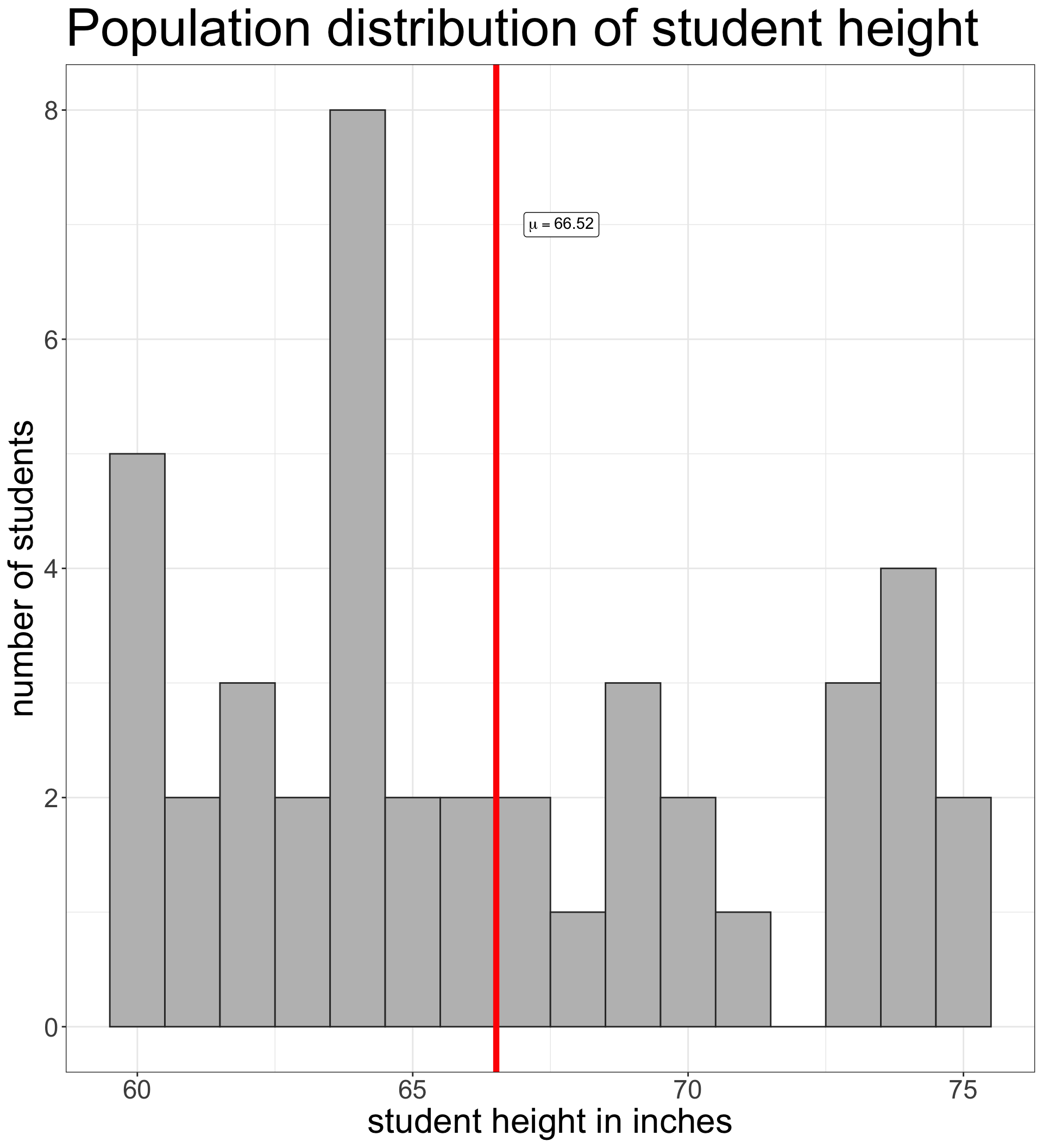
Population Distribution

The distribution of years of education for the whole US population.
Its mean is given by \(\mu\).
The population mean and distribution are unknown.

Sample Distribution

The distribution of years of education in your sample.
The mean is given by \(\bar{x}\).
The mean and distribution are known and hopefully approximate the population distribution.

Sampling Distribution

The distribution of the sample mean \(\bar{x}\) in all possible samples of size 100.
We can’t know this distribution exactly, but it turns out that we know its general shape.

Example: Height in our class

Lets treat our class of 42 students as the population. I want to estimate the average height of the class.
In this case, I am omnipotent - I know the population distribution because I collected data for the whole class on Canvas.

How many samples of size 2 are possible?

Lets say I wanted to sample two students to estimate class height. In a class of 42 students, how many unique samples of size 2 exist?

On the first draw, I have 42 possibilities.
On the second draw, I have 41 possibilities because I am not putting my first draw back.
I therefore have \(42*41=1722\) possible samples.
However, half of these samples are just duplicates of the other half, but sampled in the other order. In one sample, I samples John and Then Kate and in another I sampled Kate and then John.
Therefore the true number of unique samples is: \[42*41/2=861\]
What if I calculated the sample mean in all 861 samples and looked at the distribution of these sample means?

The sampling distribution

Sampling distributions for different \(n\)

What is the mean of the sampling distributions?

Distribution	Mean	Standard Deviation
Population Distribution	66.52	4.87
Sampling Distibution (n=2)	66.52	3.36
Sampling Distribution (n=3)	66.52	2.71
Sampling Distribution (n=4)	66.52	2.32
Sampling Distribution (n=5)	66.52	2.04

The mean of each sampling distribution equals the population mean. This is not a coincidence!
The standard deviation of the sampling distributions shrinks with sample size.

Its the Central Limit Theorem!

As the sample size increases, the sampling distribution of a sample mean becomes a normal distribution.

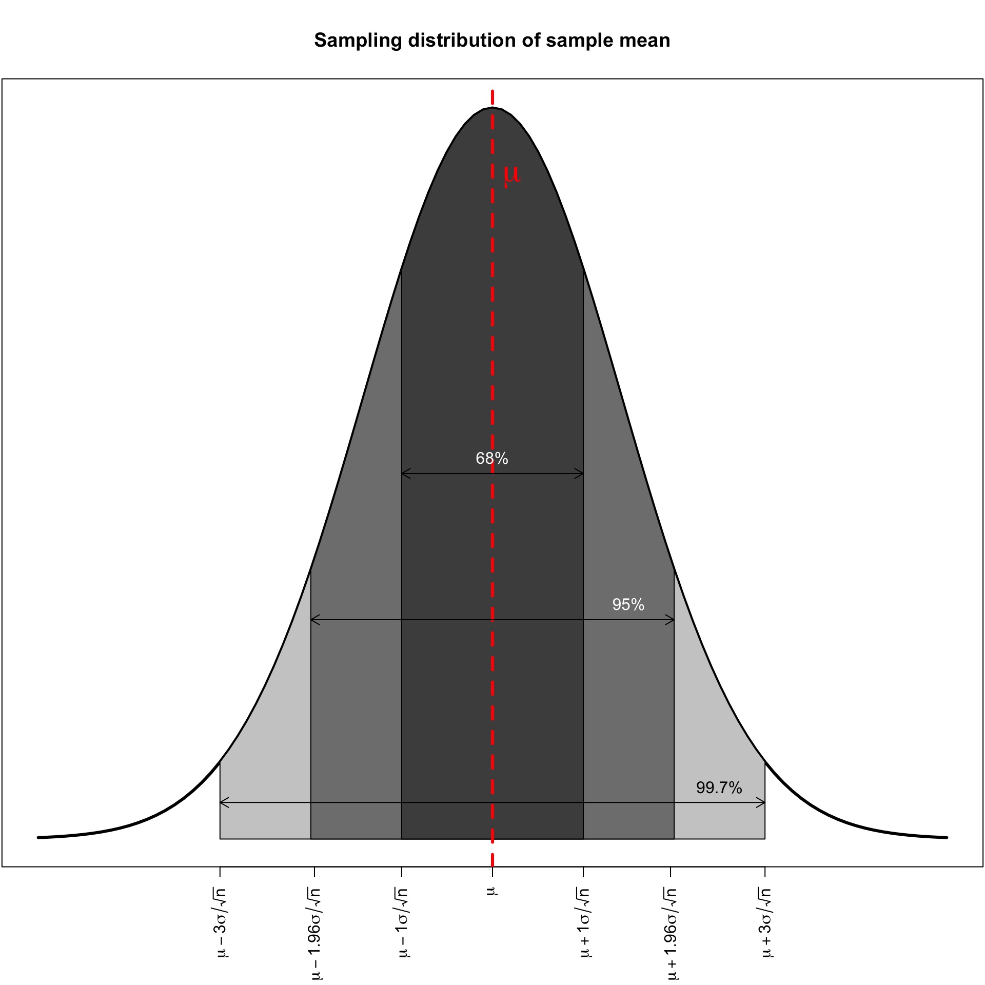
The normal distribution is a bell-shaped curve with two characteristics: center and spread.
Centered on \(\mu\), which is the true value in the population.
With a spread (standard deviation) of \(\sigma/\sqrt{n}\), where \(\sigma\) is the standard deviation in the population.
The center of the sampling distribution is the true value of the parameter and the spread of the sampling distribution shrinks as the sample grows larger.

The Standard Error

There are three different kinds of standard deviations involved here, one that corresponds to each of the types of distributions.

Distribution	Notation	Description
Population	\(\sigma\)	Unknown population standard deviation
Sample	\(s\)	Known sample standard deviation that hopefully approximates \(\sigma\)
Sampling	\(\sigma/\sqrt{n}\)	Standard error: Standard deviation of the sampling distribution

The standard error gives us an estimate of the strength of potential random bias in our sample.

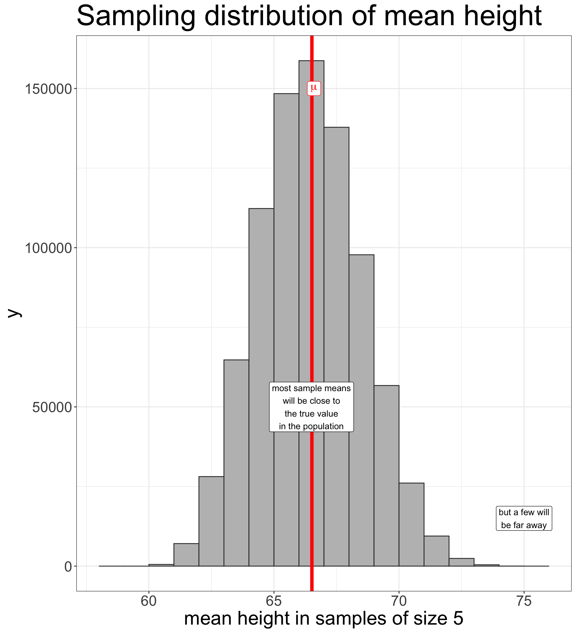
Sampling distributions are the 🔑 concept

When we draw a sample and calculate the sample mean we are effectively drawing a value from the sampling distribution for the sample mean.
If we know what that distribution looks like then we can know the probability of drawing a sample close to or far from the true population parameter.

But there is a catch!

The shape of the sampling distribution is determined by:
- the population mean, \(\mu\)
- the population standard deviation, \(\sigma\)
But these values are unknown! 😮

First Fix

We can substitute the sample standard deviation \(s\) from our sample for the population standard deviation \(\sigma\).
This has consequences. Because we are using a sample value which can also be subject to random bias, this substitution creates greater uncertainty in our estimate which we will address later.

Second Fix

Confidence Intervals: Provide a range of values within which you feel confident that the true population mean resides.
Hypothesis tests: Play a game of make believe. If the true population mean was a given value, what is the probability that I would get the sample mean value that I actually did?

Confidence Intervals

Consider this statement

Reverse the Logic

If I construct the following interval:

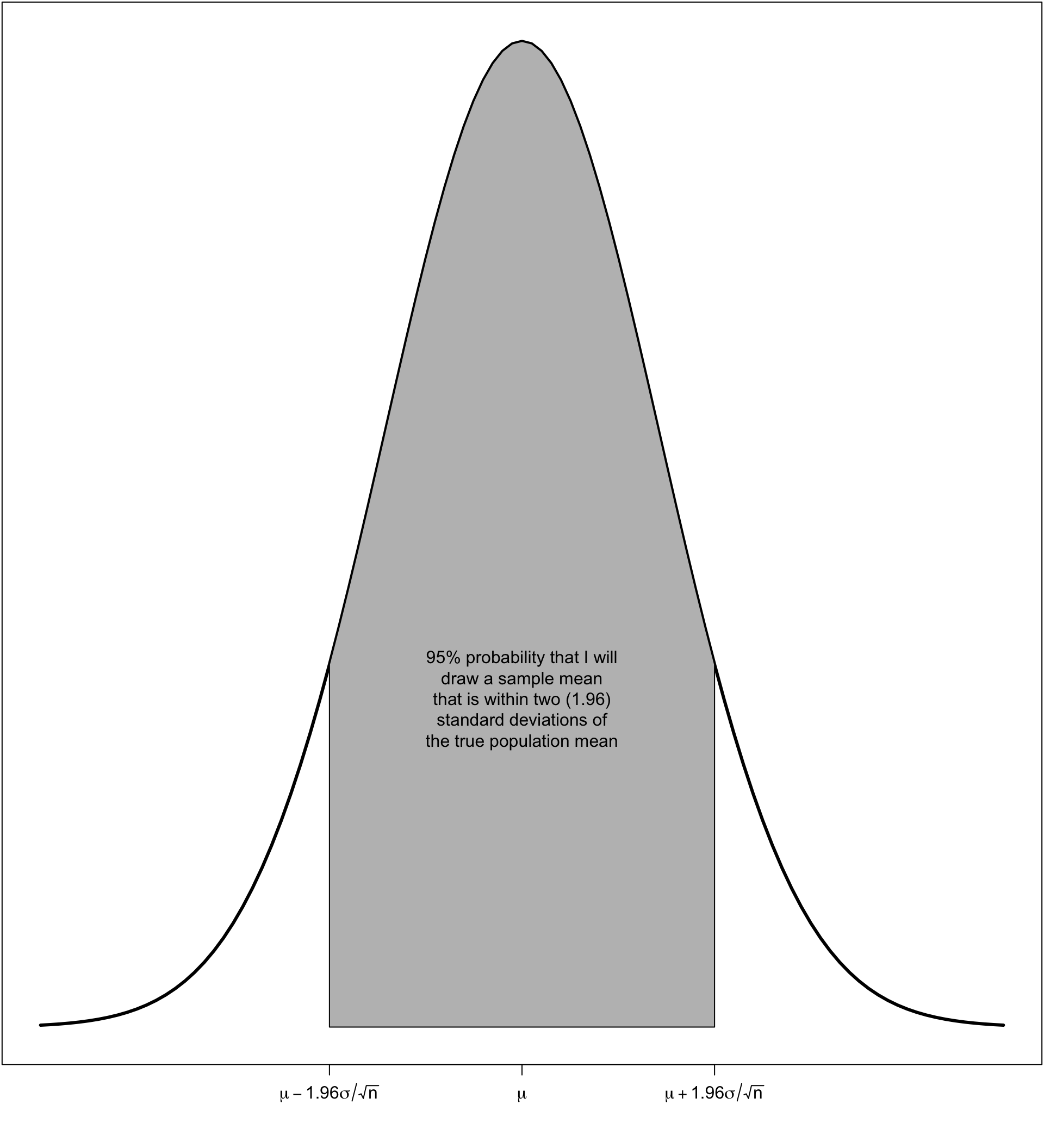
\[\bar{x}\pm1.96*\sigma/\sqrt{n}\] 95% of all possible samples that I could have drawn will contain the true population mean \(\mu\) within this interval.

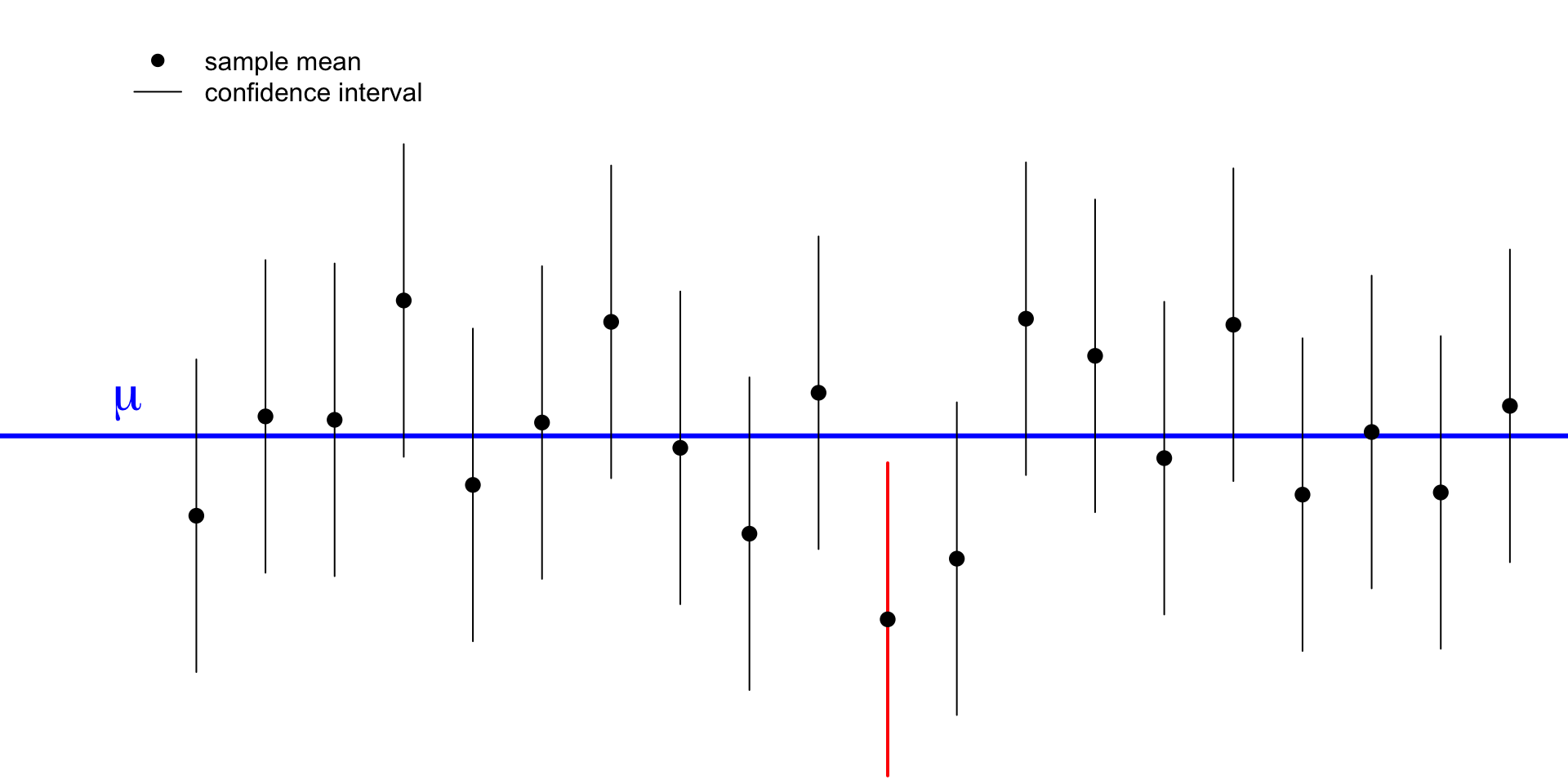
Confidence?

We call the interval of \(\bar{x}\pm1.96*\sigma/\sqrt{n}\) the confidence interval. What does it mean?

Not a probability

It is tempting to claim that there is a 95% probability that the true population mean is in this interval, but according to classic views of probability this is INCORRECT.
The true population mean does not vary. It just is what it is, even if it is unknown. Either your interval contains it or the interval does not contain it. There is no probability.
The correct interpretation is that “95% of all possible confidence intervals will contain the true population mean.”

If this seems confusing, you are normal.

Calculating the confidence interval

The confidence interval is given by \(\bar{x}\pm1.96*\sigma/\sqrt{n}\).

But we don’t know \(\sigma\) because this is the population standard deviation. What can we do?

Substitute the sample standard deviation

We can calculate \(\bar{x}\pm1.96*s/\sqrt{n}\).

However, this equation is no longer correct because we need to adjust for the added uncertainty of using a sample statistic where we should use a population parameter.

Use the t-statistic as a fudge factor

The actual formula we want is:

\[\bar{x} \pm t*s/\sqrt{n}\]

where \(t\) is the t-statistic and will be a number somewhat larger than 1.96.

Calculating the t-statistic

The t-statistic you get depends on two characteristics:

What level of confidence you want. We will always use 95% confidence intervals for this class.
The number of degrees of freedom for the statistic. This is largely a function of sample size. For the sample mean, the degrees of freedom are given by \(n-1\).

In R, you can calculate the t-statistic with the qt command. Lets say we wanted the t-statistic for our crime data with 51 observations:

qt(.975, 51-1)

[1] 2.008559

Although we want the 95% confidence interval but we need to put in 0.975, because we are getting the upper tail of the distribution which has only 2.5% of the area above.
The second argument is the degrees of freedom.

Example: Property crime rates

First we need to calculate all the statistics we need:

mean(crimes$property_rate)

[1] 2462.758

sd(crimes$property_rate)

[1] 656.6521

nrow(crimes)

[1] 51

Now we can calculate the t-statistic and standard error:

tstat <- qt(.975, 51-1)
se <- 656.6521/sqrt(51)

The upper limit is given by:

2462.758+tstat*se

[1] 2647.444

The lower limit is given by:

2462.758-tstat*se

[1] 2278.072

We are 95% confident that the true mean property crime rate across states is between 2278.1 and 2647.4 crimes per 100,000.

🤔 Wait, Does that even make sense?

We are 95% confident that the true mean property crime rate across states is between 2278.1 and 2647.4 crimes per 100,000.

We did the math right, but this statement is still nonsense. Why?

The crime data are not a sample.
We have all fifty states plus the District of Columbia. So we have the entire population.
There is nothing to infer. The mean crime rate across states of 2824 per 100,000 is already the population mean.

Statistical inference only makes sense for samples

Proper sample

Popularity data (Add Health)
Politics data (ANES)
Sexual frequency data (GSS)
Earnings data (CPS)

Not a sample

Titanic
Crimes
Movies

Example: Sexual frequency

Calculate numbers that we need for later:

xbar <- mean(sex$sexf)
s <- sd(sex$sexf)
n <- nrow(sex)
se <- s/sqrt(n)
t <- qt(.975, n-1)

	results
sample mean	46.909
sample standard deviation	44.584
sample size (n)	11785.000
standard error	0.411
t-statistic	1.960

Now calculate the interval:

xbar+t*se

[1] 47.71364

xbar-t*se

[1] 46.10359

I am 95% confident that the mean sexual frequency in the US is between 46.1 and 47.7 times per year.

General form of the confidence interval

We can construct confidence intervals for any statistic whose sampling distribution is a normal distribution. This includes:

means
mean differences
proportions
differences in proportions
correlation coefficient

The general form of the confidence interval is given by:

\[\texttt{(sample statistic)} \pm t*(\texttt{standard error})\]

The only trick is knowing how to calculate the standard error and degrees of freedom for the t-statistic for each particular statistic.

Cheat sheet for SE and df

Type	SE	df for \(t\)
Mean	\(s/\sqrt{n}\)	\(n-1\)
Proportion	\(\sqrt\frac{\hat{p}*(1-\hat{p})}{n}\)	\(n-1\)
Mean Difference	\(\sqrt{\frac{s_1^2}{n_1}+\frac{s_2^2}{n_2}}\)	min( \(n_1-1\), \(n_2-1\) )
Proportion Difference	\(\sqrt{\frac{\hat{p}_1(1-\hat{p}_1)}{n_1}+\frac{\hat{p}_2(1-\hat{p}_2)}{n_2}}\)	min( \(n_1-1\), \(n_2-1\) )
Correlation Coefficient	\(\sqrt{\frac{1-r^2}{n-2}}\)	\(n-2\)

Proportion example

What proportion of voters support removing birthright citizenship?

Use prop.table to get the sample proportion:

prop.table(table(politics$brcitizen))


   Oppose   Neither     Favor 
0.3957989 0.2860515 0.3181496

p <- 0.3181496

Calculate values:

n <- nrow(politics)
se <- sqrt(p*(1-p)/n)
t <- qt(0.975, n-1)

Get confidence intervals:

p+t*se

[1] 0.3321778

p-t*se

[1] 0.3041214

I am 95% confident that the true proportion of American adults who support removing birthright citizenship is between 30.4% and 33.2%.

Mean difference example

What is the difference in sexual frequency between married and never married individuals?

Use tapply to get means by groups and then calculate the difference you want:

tapply(sex$sexf, sex$marital, mean)

Never married       Married      Divorced       Widowed 
     53.45574      46.44548      47.87926      25.88266

diff <- 46.44548-53.45574

Use tapply again to calculate standard deviations by group for the SE calculation:

#use tapply again to get sd by group
tapply(sex$sexf, sex$marital, sd)

Never married       Married      Divorced       Widowed 
     48.06519      42.42236      46.42971      31.71475

sd1 <- 42.42236
sd2 <- 48.06519

Mean difference example, continued

Use table to get sample size by group:

table(sex$marital)


Never married       Married      Divorced       Widowed 
         3129          5374          2319           963

n1 <- 5374
n2 <- 3129

Calculate standard error, t-statistic, and confidence intervals:

se <- sqrt(sd1^2/n1+sd2^2/n2)
t <- qt(0.975,n2-1)
diff+t*se

[1] -4.979022

diff-t*se

[1] -9.041498

I am 95% confident that, among American adults, married individuals have sex between 4.98 and 9.04 fewer times per year than never married individuals, on average.

Proportion difference example

What is the difference in support for removing birthright citizenship between those who have served in the military and those who have not?

Use prop.table to calculate proportions for each group:

prop.table(table(politics$brcitizen, 
                 politics$military), 2)

         
                 No       Yes
  Oppose  0.4065643 0.3071895
  Neither 0.2893065 0.2592593
  Favor   0.3041292 0.4335512

p1 <- 0.3041292
p2 <- 0.4335512
diff <- p2-p1

Use table to get sample sizes by group:

table(politics$military)


  No  Yes 
3778  459

n1 <- 3778
n2 <- 459

Proportion difference example, continued

Calculate standard error and t-statistic:

se <- sqrt(p1*(1-p1)/n1+p2*(1-p2)/n2)
t <- qt(0.975, n2-1)

Calculate confidence intervals:

diff-t*se

[1] 0.08164563

diff+t*se

[1] 0.1771984

I am 95% confident that the percent in support for removing birthright citizenship is between 8.2% and 17.7% higher among who have served in the military than those who have not.

Correlation coefficent example

What is the correlation between age and wages among US workers?

Use cor command to get the sample correlation coefficient:

r <- cor(earnings$age, earnings$wages)

Use nrow to get sample size and then calculate standard error and t-statistic.

n <- nrow(earnings)
se <- sqrt((1-r^2)/(n-2))
t <- qt(0.975, n-2)

Calculate confidence intervals:

r - t*se

[1] 0.2135195

r + t*se

[1] 0.2235427

I am 95% confident that the true correlation coefficient between age and wages among US workers is between 0.214 and 0.224.

Hypothesis Tests

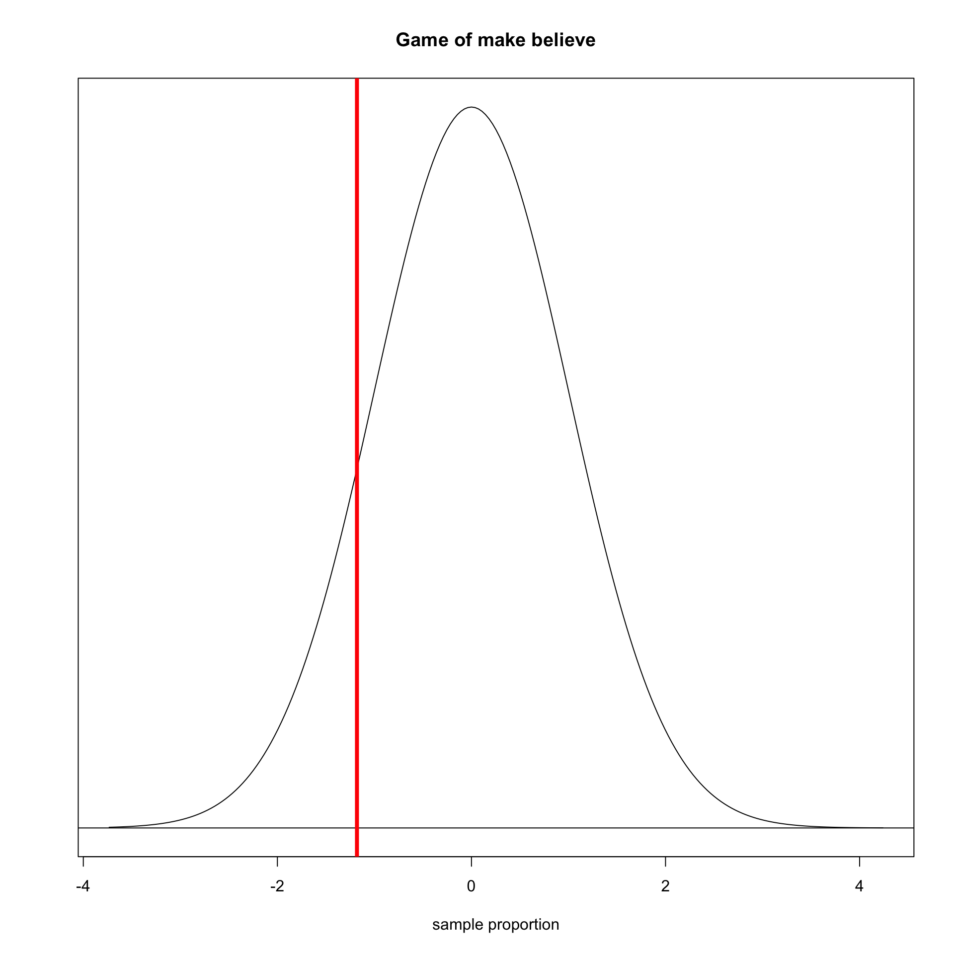
Game of make believe

We know what the sampling distribution should look like, but we don’t know its center (the true population parameter).

So we set up a game of make-believe:

Assume that the true parameter is some value.
If assumption is correct, what is the probability that I would have gotten the sample statistic that I got?
If this probability is really low, then I reject my assumption.

An almost true story

Coca-Cola used to do promotionals where it claimed that 1 in 12 bottle caps (8.3%) on a Coca-Cola bottle would earn a free Coke.
When I was a busy assistant professor trying to get tenure, I bought 100 bottles of Coke from the downstairs vending machine and only got 5 winners (5%). (The number is not true, but it is nice and round)
Does the difference between my winning percentage and that claimed by Coca-Cola show that they were lying?

Lets set up a null hypothesis

In English

The null hypothesis ( \(H_0\) ) is your assumption about the true parameter value. It is your prior assumption unless the data can prove you wrong.
I assume that Coca-Cola is telling the truth, until I can prove them wrong, so my null hypothesis is that the true percentage of winning bottlecaps is 8.3%.

Mathematical symbols

\[H_0: \rho=0.083\]

I use the Greek \(\rho\) to indicate the population proportion of winners. I will use \(\hat{p}\) later to represent the proportion observed in my sample.

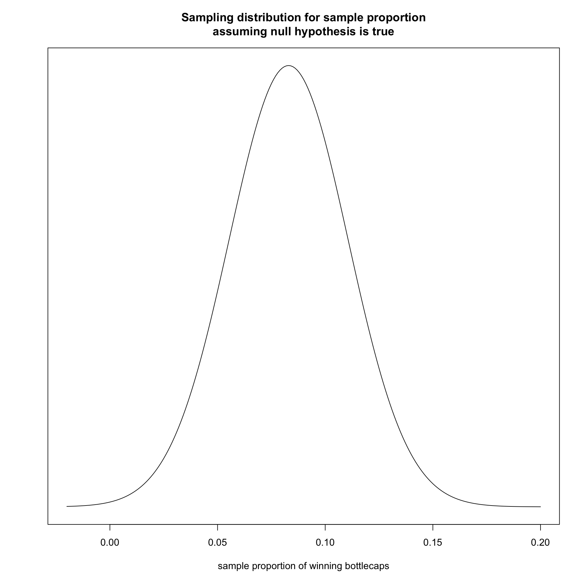
Assuming \(H_0\) is true, what is the sampling distribution of my sample proportion?

]

Assuming \(H_0\) is true, what is the sampling distribution of my sample proportion?

With a sample size of 100, it should be normally distributed.

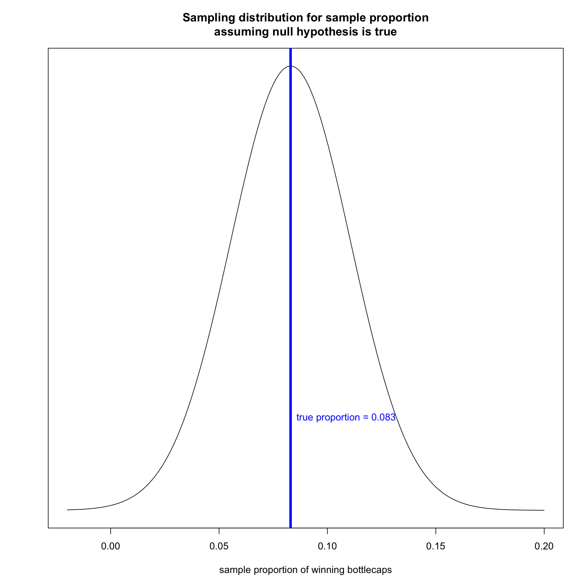
Assuming \(H_0\) is true, what is the sampling distribution of my sample proportion?

With a sample size of 100, it should be normally distributed.

The center of the distribution is the true population parameter assuming \(H_0\) is true. In this case, that is 0.083.

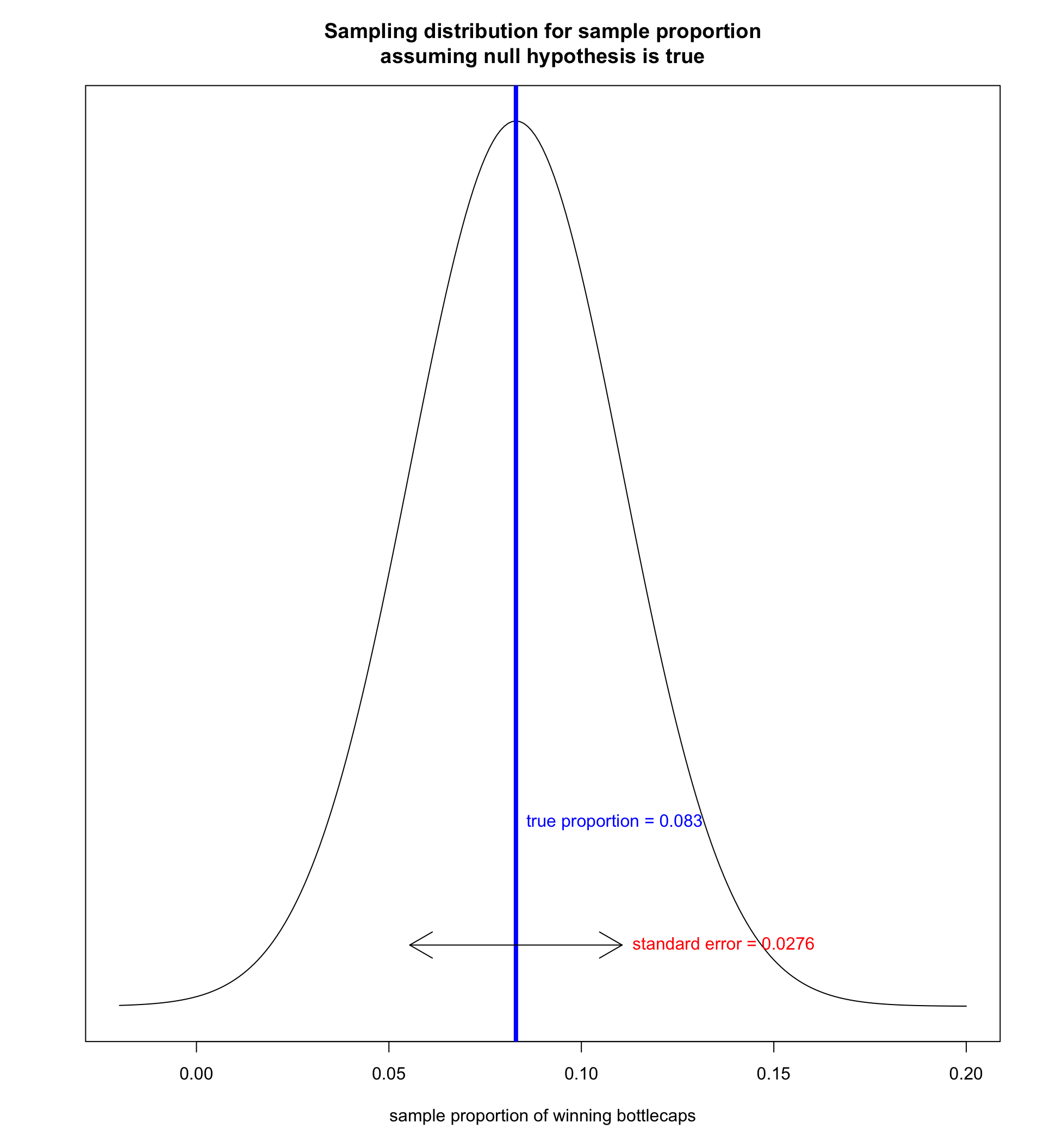
Assuming \(H_0\) is true, what is the sampling distribution of my sample proportion?

With a sample size of 100, it should be normally distributed.

The center of the distribution is the true population parameter assuming \(H_0\) is true. In this case, that is 0.083.

As we learned in the previous section, the standard error is given by: \[\sqrt\frac{0.083*(1-0.083)}{100}=0.0276\]

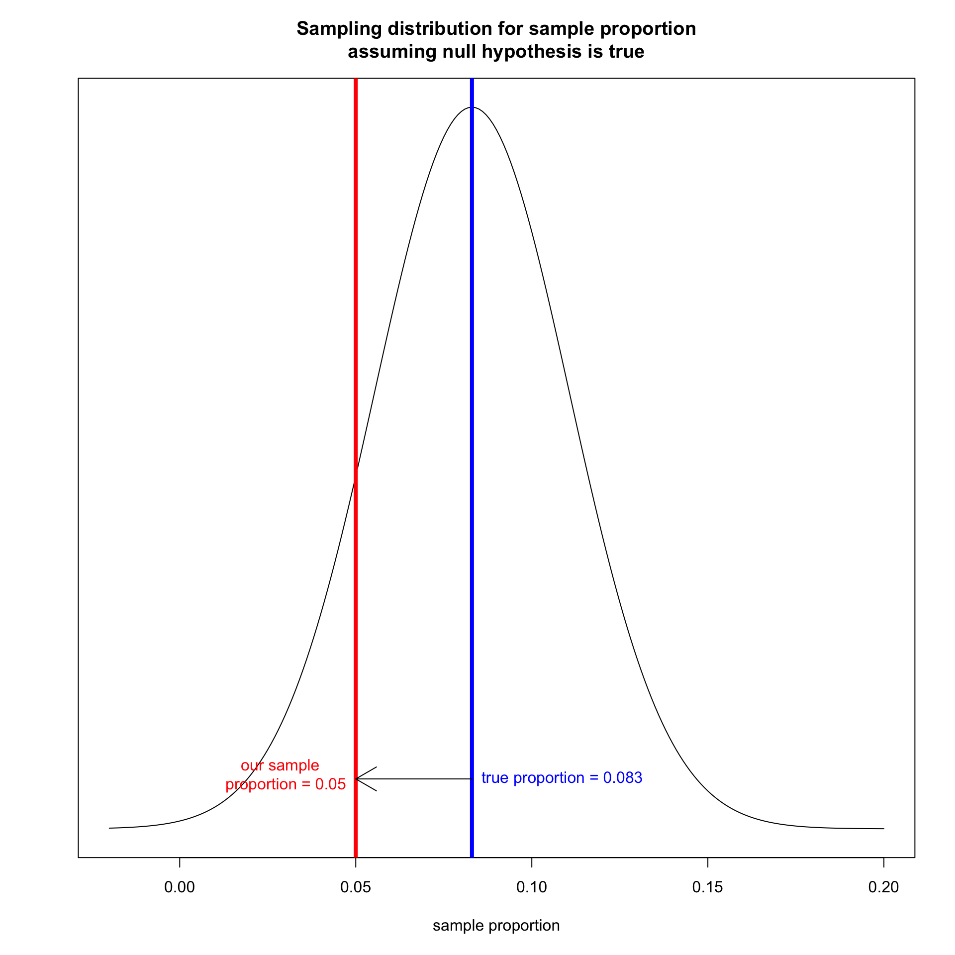
Is the actual sample proportion unusual?

How far is our sample proportion from where the center would be if the null hypothesis was true?

If our sample proportion is far way and unlikely to be drawn, then we reject the null hypothesis.
If our sample proportion is not far away and reasonably likely to be drawn, then we fail to reject the null hypothesis.

How far is far enough?

We determine how far our sample proportion is from the center in terms of the number of standard errors.

\[\frac{\hat{p}-\rho}{SE}=\frac{0.05-0.083}{0.028}=-1.18\]

How far is far enough?

We determine how far our sample proportion is from the center in terms of the number of standard errors.

\[\frac{\hat{p}-\rho}{SE}=\frac{0.05-0.083}{0.028}=-1.18\]

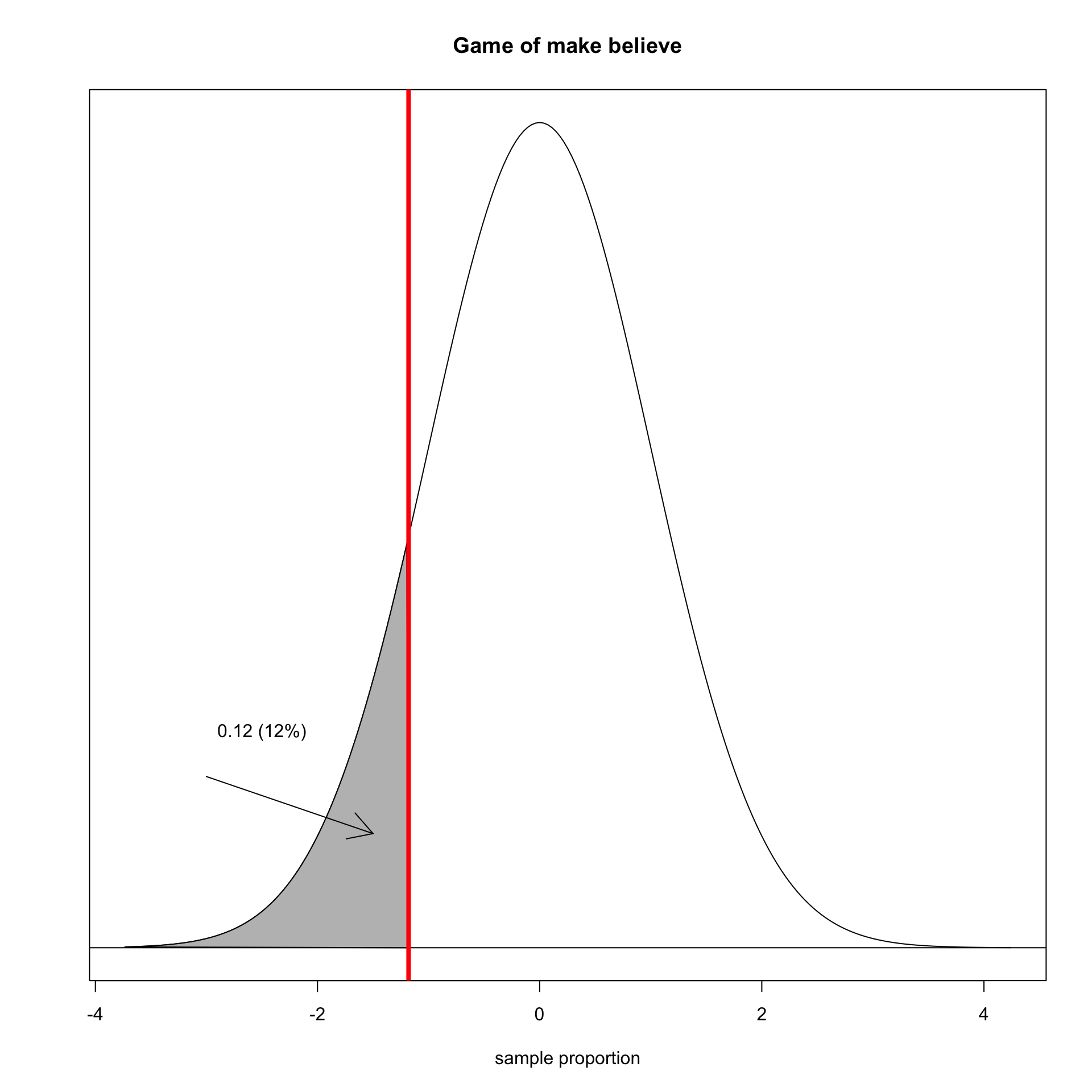
What proportion of sample proportions are this low or lower?

How far is far enough?

We determine how far our sample proportion is from the center in terms of the number of standard errors.

\[\frac{\hat{p}-\rho}{SE}=\frac{0.05-0.083}{0.028}=-1.18\]

What proportion of sample proportions are this low or lower?

We also need to take account of sample proportions this far away in the opposite direction. This is called a two-tailed test.

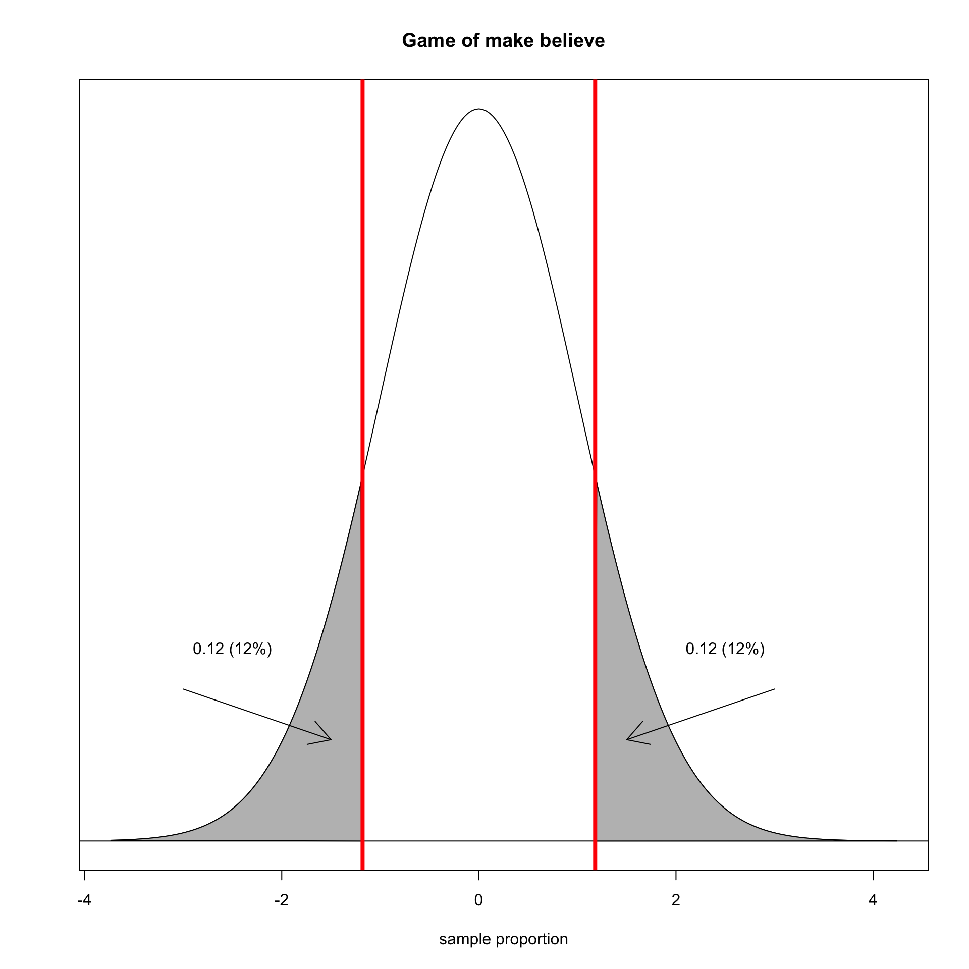
How far is far enough?

We determine how far our sample proportion is from the center in terms of the number of standard errors.

\[\frac{\hat{p}-\rho}{SE}=\frac{0.05-0.083}{0.028}=-1.18\]

What proportion of sample proportions are this low or lower?

We also need to take account of sample proportions this far away in the opposite direction. This is called a two-tailed test.

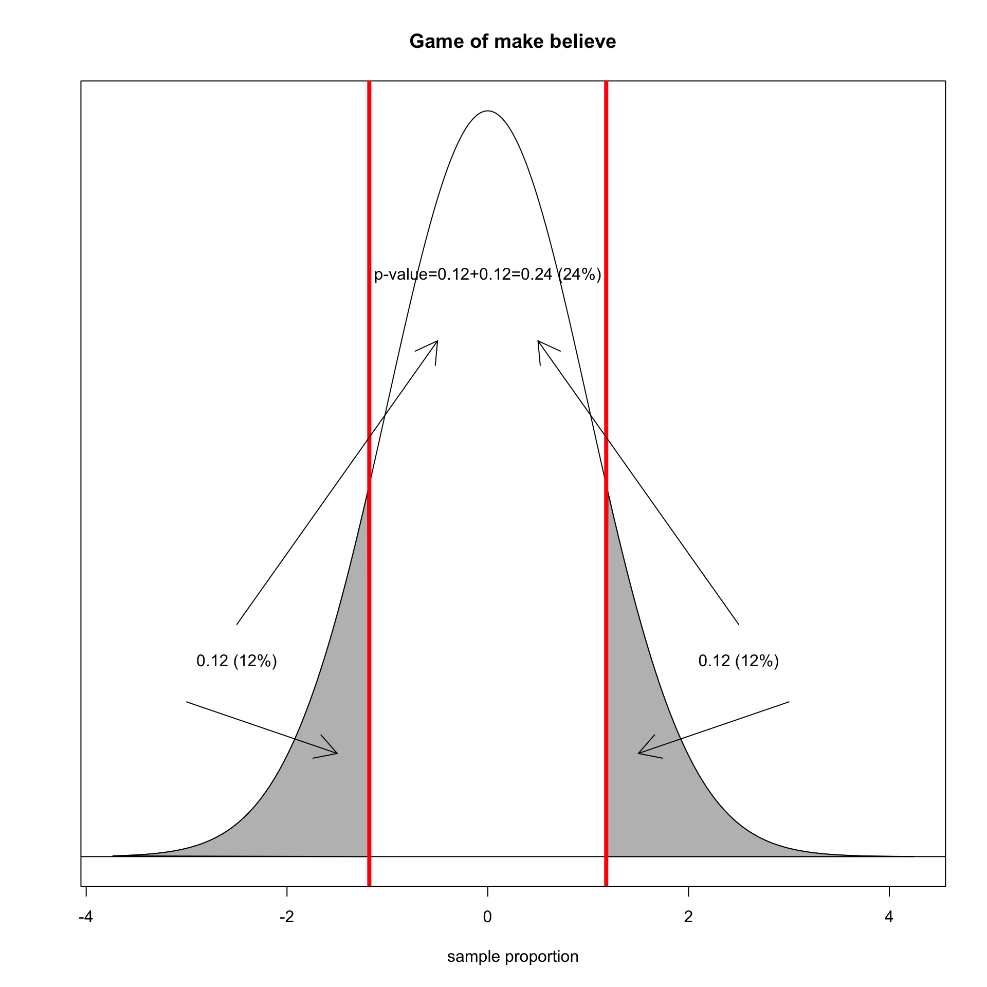
The area in the tails is called the p-value.

The p-value is the endgame

Interpretation

The p-value tells you the probability of getting a statistic this far away or farther from the the assumed true population parameter, assuming the null hypothesis is true.

In my case:

Assuming the null hypothesis is true, there is a 24% probability that I would have gotten a sample proportion (0.05) this far or farther from the true poplation paramter (0.083).

Calculation

We use the pt command to get the area in the lower tail and multiply by two to get both tails:

2*pt(-1.18,99)

[1] 0.2408278

The first argument is always the negative version of the number of standard errors away because this command will always give you the area below the value.
The second argument is the degrees of freedom to adjust for the fact that we use sample standard deviations to get standard errors.

The critical value

We will reject the null hypothesis if our p-value is low enough.
The critical value is the benchmark for how low our p-value has to be to reject.
- We will reject the null hypothesis if the p-value is lower than or equal to the critical value.
- We will fail to reject the null hypothesis if the p-value is higher than the critical value.
The standard but entirely arbitrary critical value used across the sciences is 0.05 (5%).
For the Coca-Cola bottlecap case, the p-value is 0.24, so we fail to reject the null hypothesis that Coca-Cola’s claim was truthful.

The general procedure of hypothesis testing

State a null hypothesis.
Calculate a test statistic that tells you how different your sample is from what you would expect under the null hypothesis. For our purposes, this test statistic is always the number of standard errors above or below the center of the sampling distribution.
Calculate the p-value for the given test statistic.
Based on the p-value, either reject or fail to reject the null hypothesis.

Hypothesis tests of relationships

The hypothesis test we are most interested in is whether the association we observe between two variables in our sample holds in the population.

Mean/proportion differences: Are the means/proportions between two groups in the population different? In other words, is the mean/proportion difference non-zero?
Correlation coefficient: is the correlation coefficient in the population non-zero?

Statistical Significance

If you reject the null hypothesis of “no association,” then the association you observe in the sample is said to be statistically significant.
Don’t confuse statistical and substantive significance. In a large sample, even very small substantive associations can be found to be statistically significant. On the flip side, in small samples, very large substantive associations can fail to be statistically significant.

Example: Mean differences

Is there a difference in sexual frequency between married and divorced individuals? Formally, my null hypothesis is:

\[H_0: \mu_M-\mu_D=0\]

Where \(\mu_M\) is the population mean sexual frequency of married individuals and \(\mu_D\) is the population mean sexual frequency of divorced individuals.

tapply(sex$sexf, sex$marital, mean)

Never married       Married      Divorced       Widowed 
     53.45574      46.44548      47.87926      25.88266

diff <- 46.44548-47.87926
diff

[1] -1.43378

In my sample, married individuals have sex about 1.4 fewer times per year than divorced individuals, on average. Is this difference far enough from zero to reject the null hypothesis?

I gather terms to calculate the standard error.

tapply(sex$sexf, sex$marital, sd)

Never married       Married      Divorced       Widowed 
     48.06519      42.42236      46.42971      31.71475

sd1 <- 42.42236
sd2 <- 46.42971
table(sex$marital)


Never married       Married      Divorced       Widowed 
         3129          5374          2319           963

n1 <- 5374
n2 <- 2319
se <- sqrt(sd1^2/n1+sd2^2/n2)

Example: Mean differences, continued

I can now calculate how many standard errors my sample mean difference is from zero:

diff/se

[1] -1.275052

I then feed the negative version of this number into the pt formula and multiply by two to get my p-value:

2*pt(-1.275052, n2-1)

[1] 0.2024186

Assuming that the true sexual frequency difference between married and divorced individuals is zero in the population, there is a 20.2% chance of observing a sample sexual frequency difference of 1.4 times per year or larger between the two groups in a sample of this size. Thus, I fail to reject the null hypothesis there there is no difference in the average sexual frequency between married and divorced individuals in the US.

Example: Proportion differences

Is there a difference in support for removing birthright citizenship between those who have served in the military and those who have not?

prop.table(table(politics$brcitizen, 
                 politics$military), 2)

         
                 No       Yes
  Oppose  0.4065643 0.3071895
  Neither 0.2893065 0.2592593
  Favor   0.3041292 0.4335512

p1 <- 0.304
p2 <- 0.434

diff <- p2-p1
diff

[1] 0.13

table(politics$military)


  No  Yes 
3778  459

n1 <- 3778
n2 <- 459
se <- sqrt(p1*(1-p1)/n1+p2*(1-p2)/n2)
diff/se

[1] 5.346688

2*pt(-5.346688, n2-1)

[1] 1.416426e-07

🤔 A p-value of 1.416426e-07?

What does the value of 1.416426e-07 mean?
The number is so small that R is reporting it using scientific notation: \[1.416426 x 10^{-7}\]
That means we need to move the decimal place over 7 spaces to the left. So the number is really 0.0000001416426. So I would interpret my result as:

Assuming that there is no difference in the US population between those who have served in the military and those who have not in support for removing birthright citizenship, there is less than a 0.000002% chance of observing a sample difference in proportion of 13.1% or greater by random chance in a sample of this size. Thus, I reject the null hypothesis there there is no difference in support for removing birthright citizenship between those who have served in the military and those who have not.

Example: Correlation coefficient

Is there a relationship between a person’s age and their wages in the US?

r <- cor(earnings$age, earnings$wages)
r

[1] 0.2185311

n <- nrow(earnings)
se <- sqrt((1-r^2)/(n-2))
r/se

[1] 85.46473

2*pt(-85.46473, n-2)

[1] 0

Assuming no association between a person’s age and their wage in the US, there is almost 0% chance of observing a correlation coefficient between age and wages of 0.219 or larger in absolute magnitude in a sample of this size. Therefore, I reject the null hypothesis that there is no relationship between a person’s age and their wages in the US population.